Machine Learning Algorithms

Machine Learning Algorithms: A Detailed Guide

Machine Learning (ML) is a branch of Artificial Intelligence (AI) that allows computers to learn and make predictions or decisions without being explicitly programmed. The algorithms in ML are designed to learn patterns from data and provide insights or predictions.

❉ Types of Machine Learning Algorithms

Machine learning algorithms are broadly classified into three categories:

• Supervised Learning: The model learns from labeled data (input-output pairs).
• Unsupervised Learning: The model identifies patterns in unlabeled data.
• Reinforcement Learning: The model learns by interacting with the environment to maximize a reward.

Let’s dive into the algorithms one by one.

❉ Supervised Learning Algorithms

In supervised learning, the algorithm learns from labeled data, where the input features are paired with correct output labels. The goal is to predict the output (target variable) for new, unseen data based on this learned relationship. Here, we’ll start with Linear Regression.

❉ Linear Regression

Linear regression is one of the simplest and most commonly used algorithms in supervised learning. It models the relationship between the dependent variable (target) and one or more independent variables (features) by fitting a linear equation to the observed data.

Mathematical Representation:

The equation of a straight line is: [math]y = mx + c[/math]

For multiple variables: [math]y = w_1x_1 + w_2x_2 + \dots + w_nx_n + b[/math]

Where:

• [math]y[/math]: Target variable
• [math]x_i[/math]: Independent variables (features)
• [math]w_i[/math]: Weights (coefficients)
• [math]b[/math]: Bias (intercept)

Example: Predicting House Prices

Suppose you want to predict house prices based on features like area (in square feet).
The relationship can be modeled as: [math]\text{Price} = w_1 \times \text{Area} + b[/math]

Python Implementation

Here’s how to implement Linear Regression using Python:

  # Step 1: Import necessary libraries
import numpy as np
import matplotlib.pyplot as plt
from sklearn.model_selection import train_test_split
from sklearn.linear_model import LinearRegression
from sklearn.metrics import mean_squared_error

# Step 2: Create the dataset
# Example: Predict house price based on area (in 1000 sq ft)
area = np.array([1.2, 1.5, 2.3, 2.8, 3.5]).reshape(-1, 1)  # Feature (Area)
price = np.array([200, 250, 300, 400, 500])  # Target (Price in $1000s)

# Step 3: Split the dataset into training and testing sets
X_train, X_test, y_train, y_test = train_test_split(area, price, test_size=0.2, random_state=42)

# Step 4: Train the Linear Regression model
model = LinearRegression()
model.fit(X_train, y_train)

# Step 5: Make predictions
y_pred = model.predict(X_test)

# Step 6: Evaluate the model
mse = mean_squared_error(y_test, y_pred)
print(f"Mean Squared Error: {mse:.2f}")
print(f"Model Coefficients: {model.coef_}, Intercept: {model.intercept_}")

# Step 7: Visualize the results
plt.scatter(area, price, color="blue", label="Data")
plt.plot(area, model.predict(area), color="red", label="Prediction")
plt.xlabel("Area (1000 sq ft)")
plt.ylabel("Price ($1000)")
plt.legend()
plt.show()
  📋 copy code

Output:

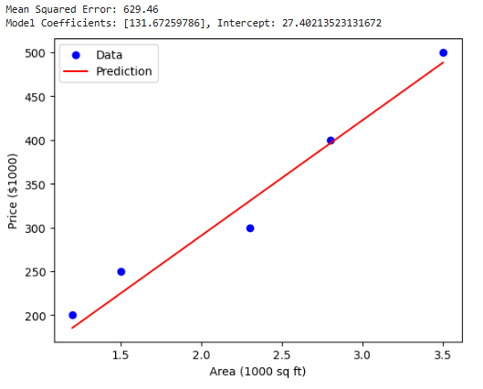
Output Explanation:

• Data Points: The scatter plot shows the actual data (blue points).
• Regression Line: The red line represents the model’s prediction.
• Model Coefficients: The slope of the line is the weight ([math]w_1[/math]), and the intercept is [math]b[/math].

Key Points About Linear Regression:

• Assumptions:
  • The relationship between features and target is linear.
  • Residuals (errors) are normally distributed.
  • No multicollinearity among features.

• When to Use:
  • Predict continuous values (e.g., house prices, salaries).
  • Analyze relationships between variables.

• Limitations:
  • Poor performance on non-linear data.
  • Sensitive to outliers.

❉ Logistic Regression

Logistic Regression is a classification algorithm used to predict discrete outcomes. Unlike Linear Regression, which predicts continuous values, Logistic Regression predicts the probability that an instance belongs to a particular class.

How It Works:

Logistic Regression uses the logistic function (also known as the sigmoid function) to map predictions to a range of 0 to 1.

The sigmoid function is given by: [math]\sigma(z) = \frac{1}{1 + e^{-z}}[/math]

Where [math]z = w_1x_1 + w_2x_2 + \dots + w_nx_n + b[/math].

The output of the sigmoid function is interpreted as a probability:

• If the probability is greater than 0.5, the instance is classified as 1.
• Otherwise, it is classified as 0.

Example: Predicting Email Spam

You have a dataset where emails are labeled as spam (1) or not spam (0). Logistic Regression can classify new emails based on features such as the number of links, length of the email, etc.

Python Implementation

  # Step 1: Import necessary libraries
import numpy as np
from sklearn.model_selection import train_test_split
from sklearn.linear_model import LogisticRegression
from sklearn.metrics import accuracy_score, confusion_matrix

# Step 2: Create the dataset
# Example: Features - [Number of Links, Length of Email], Target - Spam (1) or Not Spam (0)
features = np.array([[3, 150], [1, 50], [0, 20], [5, 300], [2, 120], [1, 100]])
target = np.array([1, 0, 0, 1, 0, 0])  # 1 = Spam, 0 = Not Spam

# Step 3: Split the dataset
X_train, X_test, y_train, y_test = train_test_split(features, target, test_size=0.3, random_state=42)

# Step 4: Train the Logistic Regression model
model = LogisticRegression()
model.fit(X_train, y_train)

# Step 5: Make predictions
y_pred = model.predict(X_test)

# Step 6: Evaluate the model
accuracy = accuracy_score(y_test, y_pred)
conf_matrix = confusion_matrix(y_test, y_pred)

print(f"Accuracy: {accuracy:.2f}")
print("Confusion Matrix:")
print(conf_matrix)

# Step 7: Interpret predictions
for i, pred in enumerate(y_pred):
    print(f"Email {i+1}: {'Spam' if pred == 1 else 'Not Spam'}")
  📋 copy code

Output:

Output Explanation:

• Accuracy: Indicates how many predictions were correct.
• Confusion Matrix: Provides a breakdown of true positives, true negatives, false positives, and false negatives.

Key Points About Logistic Regression:

• When to Use:
  • Binary classification tasks (e.g., spam detection, loan approval).
  • Multi-class classification (with extensions like softmax).

• Limitations:
  • Assumes linear decision boundaries.
  • Not suitable for complex relationships.

❉ Decision Trees

Decision Trees are versatile machine learning algorithms capable of performing both classification and regression tasks. They work by splitting the data into subsets based on feature values, forming a tree-like structure.

How It Works:

• The dataset is split at each node based on the feature that results in the maximum information gain or minimum Gini impurity.
• This process continues recursively until a stopping condition is met (e.g., maximum depth or minimum number of samples per node).

Example: Predicting Loan Approval

You want to predict whether a person’s loan application will be approved based on features like income, loan amount, and credit history.

Python Implementation

  # Step 1: Import necessary libraries
from sklearn.tree import DecisionTreeClassifier
from sklearn.metrics import accuracy_score, classification_report

# Step 2: Create the dataset
# Features - [Income, Loan Amount, Credit History (1 = Good, 0 = Bad)]
features = np.array([[50000, 200, 1], [40000, 150, 1], [30000, 100, 0], [60000, 250, 1], [35000, 120, 0]])
target = np.array([1, 1, 0, 1, 0])  # 1 = Loan Approved, 0 = Loan Rejected

# Step 3: Split the dataset
X_train, X_test, y_train, y_test = train_test_split(features, target, test_size=0.3, random_state=42)

# Step 4: Train the Decision Tree model
model = DecisionTreeClassifier(max_depth=3, random_state=42)
model.fit(X_train, y_train)

# Step 5: Make predictions
y_pred = model.predict(X_test)

# Step 6: Evaluate the model
accuracy = accuracy_score(y_test, y_pred)
print(f"Accuracy: {accuracy:.2f}")
print("Classification Report:")
print(classification_report(y_test, y_pred))
  📋 copy code

Output:

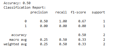
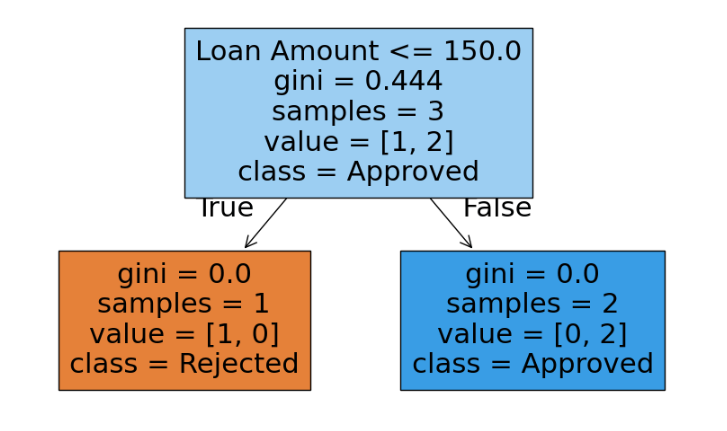
Visualization of the Decision Tree

To visualize the decision tree, use the following code:

  from sklearn.tree import plot_tree
import matplotlib.pyplot as plt

plt.figure(figsize=(10, 6))
plot_tree(model, feature_names=["Income", "Loan Amount", "Credit History"], class_names=["Rejected", "Approved"], filled=True)
plt.show()
  📋 copy code

Output:

Key Points About Decision Trees:

• Advantages:
  • Easy to interpret and visualize.
  • Handles both numerical and categorical data.

• Limitations:
  • Prone to overfitting (can be mitigated using pruning or setting maximum depth).
  • Sensitive to small changes in the data.

❉ Random Forests

Random Forest is an ensemble learning method that builds multiple decision trees and combines their predictions for better accuracy and generalization. It uses a technique called bagging, where each tree is trained on a random subset of the data.

Example: Predicting Customer Churn

You have a dataset with features like customer age, contract duration, and monthly charges. Random Forest can predict whether a customer will churn or not.

Python Implementation

  from sklearn.ensemble import RandomForestClassifier

# Step 1: Train the Random Forest model
rf_model = RandomForestClassifier(n_estimators=100, random_state=42)
rf_model.fit(X_train, y_train)

# Step 2: Make predictions
rf_y_pred = rf_model.predict(X_test)

# Step 3: Evaluate the model
rf_accuracy = accuracy_score(y_test, rf_y_pred)
print(f"Random Forest Accuracy: {rf_accuracy:.2f}")
  📋 copy code

Output: Random Forest Accuracy: 0.50

Key Points About Random Forests:

• Advantages:
  • Reduces overfitting compared to a single decision tree.
  • Handles missing data and outliers well.

• Limitations:
  • Slower than single models.
  • May require more computational resources.

❉ Support Vector Machines (SVMs)

Support Vector Machines (SVMs) are supervised learning algorithms used for both classification and regression. They aim to find the optimal hyperplane that separates data points of different classes.

How It Works:

• Hyperplane: In SVM, a hyperplane is a decision boundary that separates different classes in the feature space.
• Support Vectors: Data points closest to the hyperplane are called support vectors. These points influence the position and orientation of the hyperplane.
• Margin: SVM maximizes the margin (distance) between the hyperplane and the nearest data points of both classes.

Example: Classifying Cancer Tumors

You want to classify tumors as malignant (1) or benign (0) based on features such as tumor size and texture.

Python Implementation

  # Step 1: Import necessary libraries
from sklearn.svm import SVC
from sklearn.datasets import make_classification
from sklearn.metrics import classification_report
from sklearn.model_selection import train_test_split  # Added import

# Step 2: Create the dataset
# Generating synthetic dataset for binary classification
X, y = make_classification(n_samples=100, n_features=3, n_classes=2, n_informative=2, n_redundant=0, random_state=42)

# Step 3: Split the dataset
X_train, X_test, y_train, y_test = train_test_split(X, y, test_size=0.3, random_state=42)

# Step 4: Train the SVM model
svm_model = SVC(kernel="linear")  # Linear kernel for simplicity
svm_model.fit(X_train, y_train)

# Step 5: Make predictions
y_pred = svm_model.predict(X_test)

# Step 6: Evaluate the model
print("Classification Report:")
print(classification_report(y_test, y_pred))
  📋 copy code

Output:

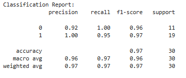
Visualizing the SVM Decision Boundary

  # Visualize the SVM Decision Boundary (using only the first two features)
import matplotlib.pyplot as plt
import numpy as np

# Create a mesh grid for visualization based on the first two features
xx, yy = np.meshgrid(np.linspace(X[:, 0].min() - 1, X[:, 0].max() + 1, 100),
                     np.linspace(X[:, 1].min() - 1, X[:, 1].max() + 1, 100))

# Predict on the grid for visualization using only the first two features
Z = svm_model.predict(np.c_[xx.ravel(), yy.ravel(), np.zeros_like(xx.ravel())])  # Set the third feature to 0
Z = Z.reshape(xx.shape)

# Plot the decision boundary
plt.contourf(xx, yy, Z, alpha=0.8, cmap=plt.cm.Paired)
plt.scatter(X[:, 0], X[:, 1], c=y, edgecolor="k", cmap=plt.cm.Paired)
plt.title("SVM Decision Boundary (Using First Two Features)")
plt.show()
  📋 copy code

Output:

Key Points About SVM:

• Advantages:
  • Effective in high-dimensional spaces.
  • Works well for small datasets.

• Limitations:
  • Not suitable for large datasets.
  • Sensitive to the choice of kernel and regularization parameter.

❉ K-Nearest Neighbors (KNN)

KNN is a simple and intuitive supervised learning algorithm. It classifies a data point based on the majority vote of its K nearest neighbors.

How It Works:

• Select the value of K (number of neighbors).
• Calculate the distance between the data point and all other points in the dataset (e.g., using Euclidean distance).
• Select the K nearest neighbors and assign the class that is most common among them.

Example: Predicting Iris Flower Species

You want to classify iris flowers into species based on features like petal length and width.

Python Implementation

  from sklearn.neighbors import KNeighborsClassifier
from sklearn.datasets import load_iris
from sklearn.metrics import accuracy_score

# Step 1: Load the Iris dataset
iris = load_iris()
X = iris.data
y = iris.target

# Step 2: Split the dataset
X_train, X_test, y_train, y_test = train_test_split(X, y, test_size=0.3, random_state=42)

# Step 3: Train the KNN model
knn_model = KNeighborsClassifier(n_neighbors=3)  # Choosing K=3
knn_model.fit(X_train, y_train)

# Step 4: Make predictions
y_pred = knn_model.predict(X_test)

# Step 5: Evaluate the model
accuracy = accuracy_score(y_test, y_pred)
print(f"Accuracy: {accuracy:.2f}")
  📋 copy code

Output: Accuracy: 1.00

Key Points About KNN:

• Advantages:
  • Simple and easy to implement.
  • No training phase (lazy learner).

• Limitations:
  • Computationally expensive for large datasets.
  • Sensitive to the choice of K and scaling of features.

❉ Naive Bayes

Naive Bayes is a probabilistic classifier based on Bayes’ Theorem. It assumes that features are independent of each other (a “naive” assumption).

Bayes’ Theorem: [math]P(A|B) = \frac{P(B|A) \cdot P(A)}{P(B)}[/math]

Where:

• [math]P(A|B)[/math]: Posterior probability (probability of A given B).
• [math]P(B|A)[/math]: Likelihood (probability of B given A).
• [math]P(A)[/math]: Prior probability of A.
• [math]P(B)[/math]: Evidence (probability of B).

Example: Classifying Sentiments

You want to classify whether a text review is positive or negative.

Python Implementation

  from sklearn.naive_bayes import MultinomialNB
from sklearn.feature_extraction.text import CountVectorizer
from sklearn.pipeline import make_pipeline

# Step 1: Create a dataset
texts = ["I love this product", "This is the worst product ever", "Amazing quality", "Terrible service"]
labels = [1, 0, 1, 0]  # 1 = Positive, 0 = Negative

# Step 2: Train the Naive Bayes model
model = make_pipeline(CountVectorizer(), MultinomialNB())
model.fit(texts, labels)

# Step 3: Make predictions
new_texts = ["Great product", "Worst experience ever"]
predictions = model.predict(new_texts)

# Step 4: Interpret predictions
for text, label in zip(new_texts, predictions):
    print(f"Text: '{text}' => Sentiment: {'Positive' if label == 1 else 'Negative'}")
  📋 copy code

Output:

Text: 'Great product' => Sentiment: Positive
Text: 'Worst experience ever' => Sentiment: Negative

Key Points About Naive Bayes:

• Advantages:
  • Works well for text classification and spam detection.
  • Fast and efficient for large datasets.

• Limitations:
  • Assumes feature independence, which may not hold in real-world data.

❉ Unsupervised Learning Algorithms

In unsupervised learning, the algorithm analyzes data without labeled outputs and aims to identify patterns or structures in the data, such as clustering similar data points or reducing dimensionality.

Here, we will cover Unsupervised Learning Algorithms such as K-Means Clustering, Hierarchical Clustering, and Principal Component Analysis (PCA).

❉ K-Means Clustering

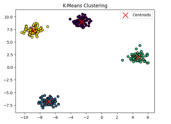
K-Means is an unsupervised learning algorithm used for clustering. It groups data points into K clusters based on their similarity.

How It Works:

• Choose the number of clusters (K).
• Randomly initialize K centroids (points representing the center of each cluster).
• Assign each data point to the nearest centroid (based on Euclidean distance).
• Recalculate the centroids by averaging the positions of the data points in each cluster.
• Repeat steps 3 and 4 until the centroids no longer change or a maximum number of iterations is reached.

Example: Grouping Customers by Spending Patterns

Suppose you have customer data (e.g., annual income and spending score), and you want to group customers into different segments.

Python Implementation

  import numpy as np
import matplotlib.pyplot as plt
from sklearn.cluster import KMeans
from sklearn.datasets import make_blobs

# Step 1: Create a synthetic dataset
X, _ = make_blobs(n_samples=300, centers=4, cluster_std=0.6, random_state=42)

# Step 2: Apply K-Means Clustering
kmeans = KMeans(n_clusters=4, random_state=42)
kmeans.fit(X)

# Step 3: Get cluster labels and centroids
labels = kmeans.labels_
centroids = kmeans.cluster_centers_

# Step 4: Visualize the clusters
plt.scatter(X[:, 0], X[:, 1], c=labels, cmap='viridis', marker='o', edgecolor='k')
plt.scatter(centroids[:, 0], centroids[:, 1], c='red', marker='x', s=200, label='Centroids')
plt.title('K-Means Clustering')
plt.legend()
plt.show()
  📋 copy code

Output:

Key Points About K-Means:

• Advantages:
  • Easy to implement.
  • Efficient for large datasets.

• Limitations:
  • Requires specifying the number of clusters (K).
  • Sensitive to the initial placement of centroids and outliers.

❉ Hierarchical Clustering

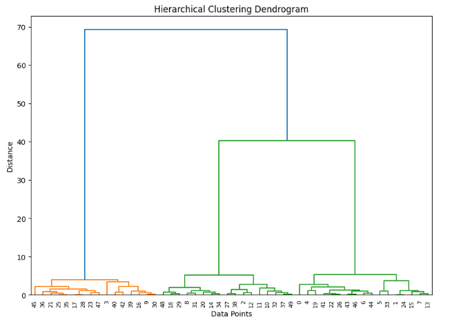
Hierarchical Clustering builds a hierarchy of clusters by either merging smaller clusters into larger ones (agglomerative) or splitting larger clusters into smaller ones (divisive).

How It Works (Agglomerative Approach):

• Treat each data point as a single cluster.
• Merge the two closest clusters based on a distance metric (e.g., Euclidean distance).
• Repeat step 2 until all points belong to one cluster or a predefined number of clusters is reached.

Example: Grouping Animals Based on Features

Suppose you want to group animals based on their size and speed.

Python Implementation

  from scipy.cluster.hierarchy import dendrogram, linkage
from sklearn.datasets import make_blobs

# Step 1: Create a synthetic dataset
X, _ = make_blobs(n_samples=50, centers=3, cluster_std=1.0, random_state=42)

# Step 2: Perform hierarchical clustering
linkage_matrix = linkage(X, method='ward')

# Step 3: Plot the dendrogram
plt.figure(figsize=(10, 7))
dendrogram(linkage_matrix)
plt.title('Hierarchical Clustering Dendrogram')
plt.xlabel('Data Points')
plt.ylabel('Distance')
plt.show()
  📋 copy code

Output:

Key Points About Hierarchical Clustering:

• Advantages:
  • No need to specify the number of clusters in advance.
  • Provides a dendrogram, which offers a visual representation of the clustering process.

• Limitations:
  • Computationally expensive for large datasets.
  • Sensitive to noise and outliers.

❉ Principal Component Analysis (PCA)

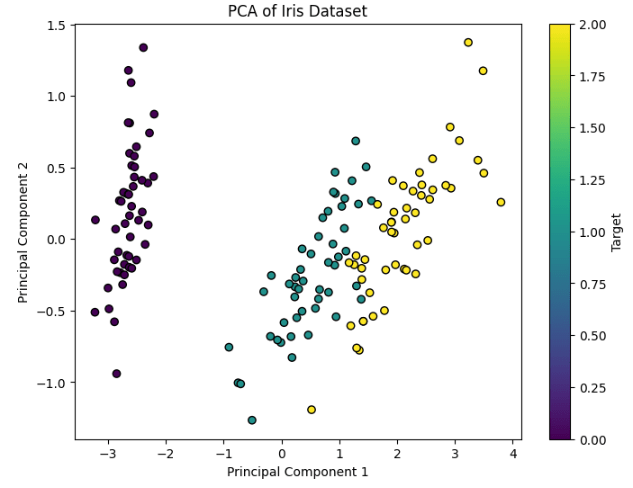
PCA is a dimensionality reduction technique that projects data onto a lower-dimensional space while preserving as much variance as possible.

How It Works:

• Standardize the dataset to have a mean of 0 and variance of 1.
• Compute the covariance matrix to understand how features are related.
• Calculate the eigenvalues and eigenvectors of the covariance matrix.
• Select the top K eigenvectors (principal components) that explain the most variance.
• Project the data onto the selected principal components.

Example: Reducing the Dimensions of Iris Dataset

Suppose you want to reduce the 4-dimensional Iris dataset to 2 dimensions for visualization.

Python Implementation

  from sklearn.decomposition import PCA
from sklearn.datasets import load_iris
import matplotlib.pyplot as plt

# Step 1: Load the Iris dataset
iris = load_iris()
X = iris.data
y = iris.target

# Step 2: Apply PCA
pca = PCA(n_components=2)  # Reduce to 2 dimensions
X_pca = pca.fit_transform(X)

# Step 3: Visualize the PCA result
plt.figure(figsize=(8, 6))
plt.scatter(X_pca[:, 0], X_pca[:, 1], c=y, cmap='viridis', edgecolor='k')
plt.xlabel('Principal Component 1')
plt.ylabel('Principal Component 2')
plt.title('PCA of Iris Dataset')
plt.colorbar(label='Target')
plt.show()
  📋 copy code

Output:

Key Points About PCA:

• Advantages:
  • Reduces the complexity of datasets.
  • Useful for visualizing high-dimensional data.

• Limitations:
  • PCA assumes linear relationships between features.
  • May lose interpretability of the original features.

❉ Advanced Machine Learning Algorithms

Here, we will cover advanced machine learning algorithms, including Random Forests, Gradient Boosting (XGBoost, LightGBM), and Neural Networks.

❉ Random Forest

Random Forest is an ensemble learning algorithm that combines the predictions of multiple decision trees to improve accuracy and reduce overfitting. It works for both classification and regression problems.

How It Works:

• Bootstrap Sampling: Randomly select subsets of data with replacement.
• Training Multiple Decision Trees: For each subset, train a decision tree using a random subset of features.
• Prediction: For classification, each tree votes for a class, and the class with the majority vote is chosen. For regression, the average prediction of all trees is taken.

Example: Predicting Iris Species

Suppose we use the Random Forest algorithm to classify Iris flowers based on their features.

Python Implementation

  from sklearn.ensemble import RandomForestClassifier
from sklearn.datasets import load_iris
from sklearn.model_selection import train_test_split
from sklearn.metrics import accuracy_score

# Step 1: Load the Iris dataset
iris = load_iris()
X = iris.data
y = iris.target

# Step 2: Split the dataset into training and testing sets
X_train, X_test, y_train, y_test = train_test_split(X, y, test_size=0.3, random_state=42)

# Step 3: Train the Random Forest model
rf = RandomForestClassifier(n_estimators=100, random_state=42)
rf.fit(X_train, y_train)

# Step 4: Make predictions
y_pred = rf.predict(X_test)

# Step 5: Evaluate the model
accuracy = accuracy_score(y_test, y_pred)
print(f"Accuracy: {accuracy * 100:.2f}%")
  📋 copy code

Output: Accuracy: 100.00%

Key Points About Random Forest:

• Advantages:
  • Reduces overfitting compared to individual decision trees.
  • Handles both classification and regression tasks.
  • Can handle missing data and outliers.

• Limitations:
  • Can be computationally expensive with large datasets.
  • The model is less interpretable compared to a single decision tree.

❉ Gradient Boosting (XGBoost, LightGBM)

Gradient Boosting is an ensemble method that builds models sequentially, where each model attempts to correct the errors made by the previous one. XGBoost and LightGBM are popular implementations of this technique, known for their speed and efficiency.

How It Works:

• Initialize a weak model (e.g., a decision tree).
• Compute the Residuals: The difference between the actual values and the predictions of the current model.
• Train a New Model: Fit a new model to the residuals (errors) of the previous model.
• Update the Model: Add the new model to the existing ensemble.
• Repeat steps 2 to 4 for a specified number of iterations.

XGBoost Example: Predicting Titanic Survival

We will use the Titanic dataset to predict whether a passenger survived based on their features (age, sex, fare, etc.).

Python Implementation (XGBoost)

  import xgboost as xgb
from sklearn.model_selection import train_test_split
from sklearn.metrics import accuracy_score
import pandas as pd

# Step 1: Load the Titanic dataset
url = 'https://raw.githubusercontent.com/datasciencedojo/datasets/master/titanic.csv'
df = pd.read_csv(url)

# Step 2: Preprocess the data
df = df[['Pclass', 'Sex', 'Age', 'Fare', 'Survived']]
df['Sex'] = df['Sex'].map({'male': 0, 'female': 1})
df['Age'].fillna(df['Age'].mean(), inplace=True)  # Handle missing values

X = df.drop('Survived', axis=1)
y = df['Survived']

# Step 3: Split the data into training and testing sets
X_train, X_test, y_train, y_test = train_test_split(X, y, test_size=0.3, random_state=42)

# Step 4: Train the XGBoost model
model = xgb.XGBClassifier(use_label_encoder=False, eval_metric='mlogloss')
model.fit(X_train, y_train)

# Step 5: Make predictions
y_pred = model.predict(X_test)

# Step 6: Evaluate the model
accuracy = accuracy_score(y_test, y_pred)
print(f"Accuracy: {accuracy * 100:.2f}%")
  📋 copy code

Output: Accuracy: 81.34%

Key Points About XGBoost and LightGBM:

• Advantages:
  • Highly efficient and fast.
  • Handles missing data and large datasets well.
  • Typically performs well in Kaggle competitions.

• Limitations:
  • Requires careful tuning of hyperparameters.
  • Can be prone to overfitting if not regularized properly.

❉ Neural Networks

Neural Networks are a class of machine learning algorithms inspired by the human brain. They consist of layers of interconnected nodes (neurons) that process input data and learn to make predictions.

How It Works:

• Input Layer: Accepts the features of the dataset.
• Hidden Layers: Apply weights, activation functions, and transformations to the input data.
• Output Layer: Produces the final prediction (e.g., class labels for classification or continuous values for regression).
• Backpropagation: The error is propagated backward through the network, and the weights are adjusted to minimize the error using gradient descent.

Example: Handwritten Digit Recognition (MNIST)

We will use a simple neural network to classify handwritten digits from the MNIST dataset.

Python Implementation (Neural Network with Keras)

  import numpy as np
from tensorflow.keras.models import Sequential
from tensorflow.keras.layers import Dense, Flatten
from tensorflow.keras.datasets import mnist
from tensorflow.keras.utils import to_categorical
from sklearn.model_selection import train_test_split

# Step 1: Load the MNIST dataset
(X, y), (_, _) = mnist.load_data()

# Step 2: Preprocess the data
X = X.astype('float32') / 255  # Normalize the pixel values to [0, 1]
y = to_categorical(y, 10)  # Convert labels to one-hot encoding

# Step 3: Split the data into training and testing sets
X_train, X_test, y_train, y_test = train_test_split(X, y, test_size=0.2, random_state=42)

# Step 4: Build the neural network model
model = Sequential()
model.add(Flatten(input_shape=(28, 28)))  # Flatten the 28x28 image into a 1D array
model.add(Dense(128, activation='relu'))  # Hidden layer with 128 neurons
model.add(Dense(10, activation='softmax'))  # Output layer with 10 neurons (one for each digit)

# Step 5: Compile the model
model.compile(optimizer='adam', loss='categorical_crossentropy', metrics=['accuracy'])

# Step 6: Train the model
model.fit(X_train, y_train, epochs=5, batch_size=32, validation_data=(X_test, y_test))

# Step 7: Evaluate the model
test_loss, test_acc = model.evaluate(X_test, y_test)
print(f"Test accuracy: {test_acc * 100:.2f}%")
  📋 copy code

Key Points About Neural Networks:

• Advantages:
  • Can model complex, non-linear relationships.
  • Works well with large datasets.
  • The architecture can be modified for different types of problems (e.g., CNNs for images, RNNs for sequences).

• Limitations:
  • Requires large amounts of data and computation power.
  • Prone to overfitting if not regularized properly.

❉ Deep Learning Algorithms

Here, we will cover Deep Learning Algorithms like Convolutional Neural Networks (CNNs), Recurrent Neural Networks (RNNs), and Autoencoders.

❉ Convolutional Neural Networks (CNNs)

Convolutional Neural Networks (CNNs) are a specialized class of neural networks designed for processing structured grid data, such as images. They are highly effective in image recognition and computer vision tasks due to their ability to learn spatial hierarchies.

How It Works:

• Convolution Layer: The core operation of a CNN, where a filter (or kernel) is convolved with the input image to extract features.
• Activation Function: Typically ReLU (Rectified Linear Unit) is applied after convolution to introduce non-linearity.
• Pooling Layer: Reduces the spatial dimensions of the image, typically using MaxPooling, to retain the most important information and reduce computation.
• Fully Connected Layer: After several convolution and pooling layers, the output is flattened and passed through fully connected layers for classification or regression.

Example: Image Classification with CNN (CIFAR-10 Dataset)

We will use a CNN to classify images from the CIFAR-10 dataset, which consists of 60,000 32×32 color images in 10 different classes.

Python Implementation (CNN with Keras)

  import tensorflow as tf
from tensorflow.keras.models import Sequential
from tensorflow.keras.layers import Conv2D, MaxPooling2D, Flatten, Dense
from tensorflow.keras.datasets import cifar10
from tensorflow.keras.utils import to_categorical

# Step 1: Load and preprocess the CIFAR-10 dataset
(X_train, y_train), (X_test, y_test) = cifar10.load_data()
X_train, X_test = X_train / 255.0, X_test / 255.0  # Normalize the pixel values
y_train, y_test = to_categorical(y_train, 10), to_categorical(y_test, 10)

# Step 2: Build the CNN model
model = Sequential([
    Conv2D(32, (3, 3), activation='relu', input_shape=(32, 32, 3)),  # Convolution layer
    MaxPooling2D((2, 2)),  # Max pooling
    Conv2D(64, (3, 3), activation='relu'),  # Second convolution layer
    MaxPooling2D((2, 2)),  # Max pooling
    Flatten(),  # Flatten the 2D matrix to 1D
    Dense(64, activation='relu'),  # Fully connected layer
    Dense(10, activation='softmax')  # Output layer for classification
])

# Step 3: Compile the model
model.compile(optimizer='adam', loss='categorical_crossentropy', metrics=['accuracy'])

# Step 4: Train the model
model.fit(X_train, y_train, epochs=10, batch_size=64, validation_data=(X_test, y_test))

# Step 5: Evaluate the model
test_loss, test_acc = model.evaluate(X_test, y_test)
print(f"Test accuracy: {test_acc * 100:.2f}%")
  📋 copy code

Key Points About CNNs:

• Advantages:
  • Excellent for image data and computer vision tasks.
  • Automatically learns relevant features from images (no need for manual feature extraction).
  • Efficient in terms of parameters due to shared weights in convolution layers.

• Limitations:
  • Can be computationally intensive, especially with large datasets and deep architectures.
  • Requires a lot of data for training to avoid overfitting.

❉ Recurrent Neural Networks (RNNs)

Recurrent Neural Networks (RNNs) are a class of neural networks designed for sequential data, such as time series, text, and speech. They have a feedback loop that allows information to be passed from one step to the next, making them well-suited for sequence modeling.

How It Works:

• Input Layer: The network processes the data in sequences, one element at a time.
• Hidden State: At each time step, the RNN maintains a hidden state that captures information about previous time steps.
• Output: After processing the entire sequence, the RNN produces an output, which can be used for classification, regression, or prediction tasks.

Example: Sentiment Analysis with RNN (IMDB Dataset)

We will use an RNN for sentiment analysis on the IMDB movie reviews dataset. The goal is to classify movie reviews as positive or negative.

Python Implementation (RNN with Keras)

  import tensorflow as tf
from tensorflow.keras.models import Sequential
from tensorflow.keras.layers import SimpleRNN, Dense, Embedding
from tensorflow.keras.datasets import imdb
from tensorflow.keras.preprocessing.sequence import pad_sequences

# Step 1: Load and preprocess the IMDB dataset
max_features = 10000  # Limit the number of words to 10,000
(X_train, y_train), (X_test, y_test) = imdb.load_data(num_words=max_features)
X_train = pad_sequences(X_train, maxlen=500)  # Pad sequences to a fixed length
X_test = pad_sequences(X_test, maxlen=500)

# Step 2: Build the RNN model
model = Sequential([
    Embedding(input_dim=max_features, output_dim=128, input_length=500),  # Embedding layer
    SimpleRNN(128, activation='relu'),  # RNN layer with 128 units
    Dense(1, activation='sigmoid')  # Output layer for binary classification (positive/negative)
])

# Step 3: Compile the model
model.compile(optimizer='adam', loss='binary_crossentropy', metrics=['accuracy'])

# Step 4: Train the model
model.fit(X_train, y_train, epochs=5, batch_size=64, validation_data=(X_test, y_test))

# Step 5: Evaluate the model
test_loss, test_acc = model.evaluate(X_test, y_test)
print(f"Test accuracy: {test_acc * 100:.2f}%")
  📋 copy code

Key Points About RNNs:

• Advantages:
  • Excellent for sequential data like time series, text, and speech.
  • Can capture temporal dependencies in data.

• Limitations:
  • Traditional RNNs suffer from vanishing/exploding gradient problems.
  • Training can be slow, especially for long sequences.

❉ Autoencoders

Autoencoders are unsupervised neural networks used for data compression, noise reduction, and feature extraction. They consist of two parts: an encoder, which compresses the data, and a decoder, which reconstructs the data from the compressed form.

How It Works:

• Encoder: Compresses the input into a lower-dimensional space (latent space).
• Decoder: Reconstructs the original input from the compressed representation.
• Loss Function: The network is trained to minimize the difference between the input and the reconstructed output (e.g., Mean Squared Error).

Example: Denoising Autoencoder

We will create a denoising autoencoder to remove noise from images, using the MNIST dataset.

Python Implementation (Autoencoder with Keras)

  import tensorflow as tf
from tensorflow.keras.models import Model
from tensorflow.keras.layers import Input, Dense
from tensorflow.keras.datasets import mnist

# Step 1: Load and preprocess the MNIST dataset
(X_train, _), (X_test, _) = mnist.load_data()
X_train, X_test = X_train / 255.0, X_test / 255.0  # Normalize the pixel values
X_train = X_train.reshape(-1, 28*28)
X_test = X_test.reshape(-1, 28*28)

# Add noise to the data (denoising task)
import numpy as np
noise_factor = 0.5
X_train_noisy = X_train + noise_factor * np.random.randn(*X_train.shape)
X_test_noisy = X_test + noise_factor * np.random.randn(*X_test.shape)

# Clip the values to be between 0 and 1
X_train_noisy = np.clip(X_train_noisy, 0., 1.)
X_test_noisy = np.clip(X_test_noisy, 0., 1.)

# Step 2: Build the autoencoder model
input_img = Input(shape=(28*28,))
encoded = Dense(128, activation='relu')(input_img)
decoded = Dense(28*28, activation='sigmoid')(encoded)

autoencoder = Model(input_img, decoded)

# Step 3: Compile and train the model
autoencoder.compile(optimizer='adam', loss='mean_squared_error')
autoencoder.fit(X_train_noisy, X_train, epochs=10, batch_size=256, validation_data=(X_test_noisy, X_test))

# Step 4: Evaluate the model
decoded_imgs = autoencoder.predict(X_test_noisy)
  📋 copy code

Key Points About Autoencoders:

• Advantages:
  • Great for unsupervised tasks like data denoising and dimensionality reduction.
  • Can be used for anomaly detection and feature extraction.

• Limitations:
  • May not perform well on highly complex data without proper architecture tuning.
  • Requires careful selection of latent space dimensionality.

❉ Generative Adversarial Networks (GANs)

Generative Adversarial Networks (GANs) are a class of deep learning algorithms used for generating new data samples that resemble a given training dataset. GANs consist of two networks: a generator and a discriminator.

• Generator: This network generates fake data (images, sounds, etc.) from random noise.
• Discriminator: This network attempts to distinguish between real data (from the training set) and fake data (produced by the generator).

The two networks are trained simultaneously in a game-like scenario where the generator tries to fool the discriminator, and the discriminator tries to correctly identify real vs. fake data.

How It Works:

• The generator creates fake data, starting from random noise.
• The discriminator evaluates the data and decides if it’s real or fake.
• Both networks are trained iteratively, with the goal of improving the generator’s ability to produce realistic data and the discriminator’s ability to distinguish between real and fake data.

Example: GAN for Image Generation (Fashion MNIST)

In this example, we will use GANs to generate images similar to the Fashion MNIST dataset, which contains grayscale images of clothing items.

Python Implementation (GAN with Keras)

  import tensorflow as tf
from tensorflow.keras.models import Sequential
from tensorflow.keras.layers import Dense, LeakyReLU
from tensorflow.keras.optimizers import Adam
from tensorflow.keras.datasets import fashion_mnist
import numpy as np
import matplotlib.pyplot as plt

# Step 1: Load and preprocess the Fashion MNIST dataset
(X_train, _), (_, _) = fashion_mnist.load_data()
X_train = X_train / 255.0  # Normalize the data
X_train = X_train.reshape(-1, 28*28)

# Step 2: Build the Generator model
def build_generator():
    model = Sequential([
        Dense(128, input_dim=100),
        LeakyReLU(0.2),
        Dense(784, activation='sigmoid'),
        Reshape((28, 28))
    ])
    return model

# Step 3: Build the Discriminator model
def build_discriminator():
    model = Sequential([
        Flatten(input_shape=(28, 28)),
        Dense(128),
        LeakyReLU(0.2),
        Dense(1, activation='sigmoid')
    ])
    return model

# Step 4: Build the GAN model
def build_gan(generator, discriminator):
    discriminator.trainable = False  # Freeze the discriminator when training the generator
    model = Sequential([generator, discriminator])
    return model

# Step 5: Compile the models
discriminator = build_discriminator()
discriminator.compile(optimizer=Adam(lr=0.0002, beta_1=0.5), loss='binary_crossentropy', metrics=['accuracy'])

generator = build_generator()

gan = build_gan(generator, discriminator)
gan.compile(optimizer=Adam(lr=0.0002, beta_1=0.5), loss='binary_crossentropy')

# Step 6: Train the GAN
epochs = 10000
batch_size = 128
half_batch = batch_size // 2

for epoch in range(epochs):
    # Train the discriminator
    idx = np.random.randint(0, X_train.shape[0], half_batch)
    real_imgs = X_train[idx]
    real_labels = np.ones((half_batch, 1))  # Label for real images
    fake_imgs = generator.predict(np.random.randn(half_batch, 100))
    fake_labels = np.zeros((half_batch, 1))  # Label for fake images

    discriminator_loss_real = discriminator.train_on_batch(real_imgs, real_labels)
    discriminator_loss_fake = discriminator.train_on_batch(fake_imgs, fake_labels)
    discriminator_loss = 0.5 * np.add(discriminator_loss_real, discriminator_loss_fake)

    # Train the generator
    noise = np.random.randn(batch_size, 100)
    valid_labels = np.ones((batch_size, 1))  # The generator aims to fool the discriminator
    generator_loss = gan.train_on_batch(noise, valid_labels)

    # Print progress
    if epoch % 1000 == 0:
        print(f"Epoch {epoch}/{epochs}, Discriminator Loss: {discriminator_loss[0]}, Generator Loss: {generator_loss}")
        if epoch % 5000 == 0:
            noise = np.random.randn(16, 100)
            generated_images = generator.predict(noise)
            plt.figure(figsize=(4, 4))
            for i in range(generated_images.shape[0]):
                plt.subplot(4, 4, i+1)
                plt.imshow(generated_images[i], cmap='gray')
                plt.axis('off')
            plt.show()
  📋 copy code

Key Points About GANs:

• Advantages:
  • Powerful for generating realistic synthetic data, such as images, videos, and audio.
  • Useful for tasks like image generation, data augmentation, and anomaly detection.

• Limitations:
  • Training can be unstable and require careful tuning.
  • Often requires a large amount of training data.

❉ Transfer Learning

Transfer learning is a machine learning technique where a model developed for a particular task is reused as the starting point for a model on a second task. It is commonly used in deep learning, especially for computer vision tasks, to leverage pre-trained models and fine-tune them for specific use cases.

How It Works:

• A pre-trained model is used as a feature extractor. The weights of the model are frozen, and only the final layer is retrained for the new task.
• The new task can benefit from the knowledge the pre-trained model has gained from the original task, which significantly reduces the training time.

Example: Image Classification with Transfer Learning (Using VGG16)

In this example, we will use a pre-trained VGG16 model, which is a popular CNN architecture, to classify new images. We’ll use transfer learning by fine-tuning VGG16 on a new dataset (e.g., Cats vs. Dogs).

Python Implementation (Transfer Learning with VGG16)

  import tensorflow as tf
from tensorflow.keras.models import Sequential
from tensorflow.keras.layers import Flatten, Dense
from tensorflow.keras.applications import VGG16
from tensorflow.keras.preprocessing.image import ImageDataGenerator
from tensorflow.keras.optimizers import Adam

# Step 1: Load the VGG16 model pre-trained on ImageNet (without the top layer)
base_model = VGG16(weights='imagenet', include_top=False, input_shape=(150, 150, 3))

# Step 2: Freeze the base model layers
base_model.trainable = False

# Step 3: Create a new model using VGG16 as the base
model = Sequential([
    base_model,
    Flatten(),
    Dense(512, activation='relu'),
    Dense(1, activation='sigmoid')  # Binary classification (cats vs dogs)
])

# Step 4: Compile the model
model.compile(optimizer=Adam(lr=0.0001), loss='binary_crossentropy', metrics=['accuracy'])

# Step 5: Prepare the data using ImageDataGenerator for data augmentation
train_datagen = ImageDataGenerator(rescale=1./255, shear_range=0.2, zoom_range=0.2, horizontal_flip=True)
test_datagen = ImageDataGenerator(rescale=1./255)

train_generator = train_datagen.flow_from_directory('data/train', target_size=(150, 150), batch_size=32, class_mode='binary')
validation_generator = test_datagen.flow_from_directory('data/validation', target_size=(150, 150), batch_size=32, class_mode='binary')

# Step 6: Train the model
model.fit(train_generator, epochs=10, validation_data=validation_generator)

# Step 7: Evaluate the model
test_loss, test_acc = model.evaluate(validation_generator)
print(f"Test accuracy: {test_acc * 100:.2f}%")
  📋 copy code

Key Points About Transfer Learning:

• Advantages:
  • Speeds up the training process significantly.
  • Reduces the need for large datasets for the new task.
  • Can improve performance by leveraging knowledge from related tasks.

• Limitations:
  • The pre-trained model may not always transfer well to tasks that are very different from the original task.
  • Requires a careful choice of which layers to freeze and fine-tune.

❉ Conclusion

In this post, we’ve covered several key machine learning algorithms, including traditional algorithms like Decision Trees and SVMs, as well as modern deep learning techniques like CNNs, RNNs, GANs, and Transfer Learning. Each of these algorithms serves a unique purpose, and the choice of which algorithm to use depends on the nature of the data and the specific task at hand.